
Snitchnotes Team
How to Analyze a Graph When Supply and Demand Both Shift
How to Analyze a Graph When Supply and Demand Both Shift
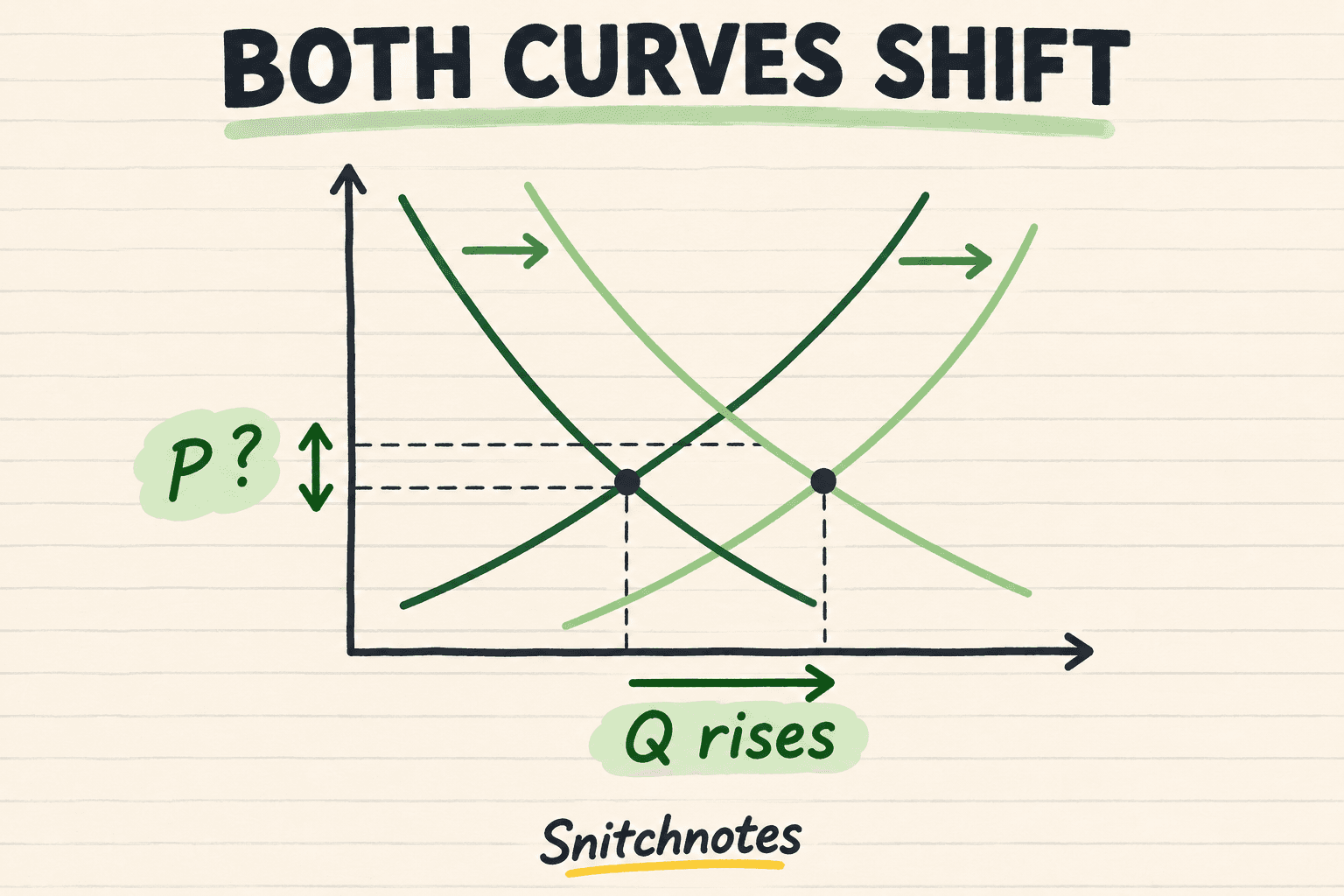
When supply and demand both shift, analyze each shift separately and compare their effects on equilibrium price and quantity. If both curves shift right, quantity definitely rises but price is ambiguous. If both shift left, quantity definitely falls but price is ambiguous. If the curves shift in opposite directions, price is certain while quantity is ambiguous. Without the relative size of the shifts, the honest answer for the conflicted outcome is “indeterminate,” not a guess.
This matters because simultaneous-shift questions are designed to test reasoning, not artistic confidence. A graph can look as if one curve moved farther simply because you drew it that way. Unless the question gives magnitudes, equations, or a scaled diagram, your sketch should reveal which forces agree and which compete—not invent missing evidence.
Start from the old equilibrium
The old equilibrium is where the original downward-sloping demand curve and upward-sloping supply curve intersect. That point gives the initial equilibrium price and quantity. A change in a non-price determinant—such as consumer preferences, income, input costs, technology, or the number of sellers—shifts an entire curve rather than causing movement along it.
Keep the two ideas separate. A higher market price causes movement along an existing supply or demand curve. A bumper harvest changes how much coffee producers can offer at every price, so supply shifts. A new taste for specialty coffee changes how much buyers want at every price, so demand shifts.
A direction-first troubleshooting method
- Identify the market. Name the exact good or service and the time period; otherwise you may shift a curve for the wrong market.
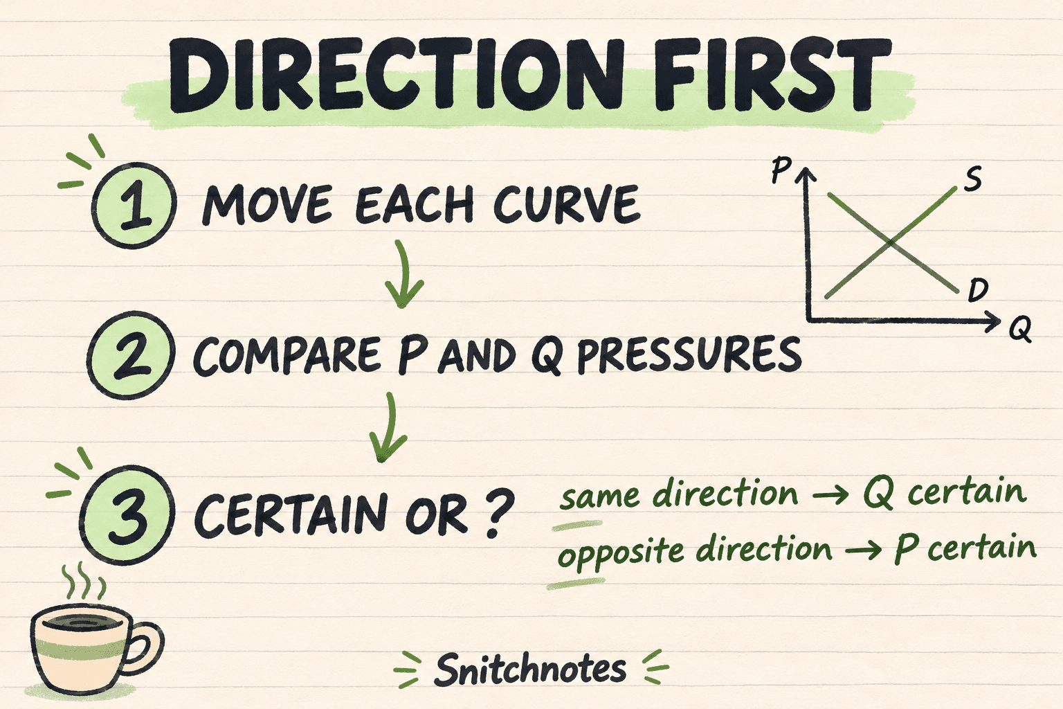
- Move each curve independently. Demand rises by shifting right and falls by shifting left. Supply rises by shifting right and falls by shifting left.
- Write each shift’s pressure on equilibrium. Demand right pushes price and quantity up; demand left pushes both down. Supply right pushes price down and quantity up; supply left pushes price up and quantity down.
- Compare the two pressures for price, then for quantity. Agreement gives a certain direction. Conflict gives an ambiguous direction unless relative magnitudes are known.
The final step is the one students often skip. Do not ask only, “Where is the new intersection on my sketch?” Ask, “Do both shifts push this outcome the same way?” Your drawn intersection is evidence only when the problem provides enough information to place it.
The four simultaneous-shift cases
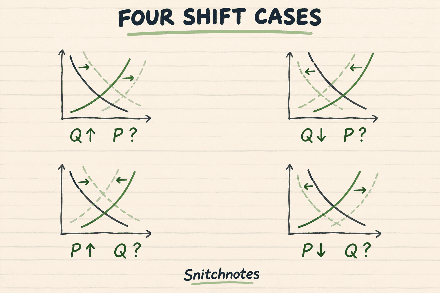
- Demand rises and supply rises: equilibrium quantity rises; equilibrium price is ambiguous.
- Demand falls and supply falls: equilibrium quantity falls; equilibrium price is ambiguous.
- Demand rises and supply falls: equilibrium price rises; equilibrium quantity is ambiguous.
- Demand falls and supply rises: equilibrium price falls; equilibrium quantity is ambiguous.
There is a compact pattern underneath all four cases. When the curves shift in the same horizontal direction, their quantity effects agree and their price effects fight. When the curves shift in opposite horizontal directions, their price effects agree and their quantity effects fight. “Ambiguous” means the model needs more information; it does not mean economics has no answer.
Coffee example: demand and supply both rise
Suppose a popular health report increases demand for coffee while a bumper harvest increases supply. Demand shifts right because buyers want more coffee at each price. Supply also shifts right because growers can offer more coffee at each price. Both shifts push equilibrium quantity upward, so more coffee is sold for sure.
Price receives conflicting pressure. Stronger demand pushes it up, while greater supply pushes it down. If the demand increase is relatively larger, the new equilibrium has a higher price. If the supply increase is relatively larger, the new price is lower. If their price effects happen to balance, the equilibrium price can stay unchanged.
Two shift sizes, two price outcomes
A small numerical model makes the boundary visible. Begin with demand Qd = 100 − 2P and supply Qs = 20 + 2P. Setting Qd equal to Qs gives an initial equilibrium of P = 20 and Q = 60. Now let demand rise to Qd = 120 − 2P.
With a modest supply increase to Qs = 30 + 2P, the new equilibrium is P = 22.5 and Q = 75: price and quantity both rise. With a larger supply increase to Qs = 50 + 2P, the new equilibrium is P = 17.5 and Q = 85: quantity still rises, but price falls. The direction of quantity survives both versions; the direction of price depends on the relative shifts.
Common mistakes and boundaries
The most common mistake is treating an unscaled sketch as data. A second is confusing an increase in supply with an increase in quantity supplied; only the first shifts the curve. A third is analyzing the events sequentially and reporting the temporary intersection after the first shift as the final result. The final equilibrium must reflect both changes together.
The shortcut also has boundaries. It assumes the standard competitive-market graph with downward demand and upward supply. If the problem gives equations, elasticities, exact changes, or a carefully scaled graph, use them to resolve the ambiguous outcome. If it involves price controls, taxes, expectations feeding back over time, or nonstandard curves, more analysis may be needed.
Check your understanding
Demand falls while supply rises. What is certain?
Equilibrium price falls because both shifts push price downward. Quantity is ambiguous: lower demand pushes it down, while higher supply pushes it up.
Demand and supply both fall. What is certain?
Equilibrium quantity falls because both shifts reduce quantity. Price is ambiguous because lower demand pushes price down while lower supply pushes it up.
When can you resolve an ambiguous outcome?
You can resolve it when the problem supplies enough information about relative magnitudes, such as equations, numerical changes, elasticities, or a graph explicitly drawn to scale.
Related concepts
- Comparative statics: comparing an initial equilibrium with a new equilibrium after an outside condition changes.
- Ceteris paribus: holding other relevant factors constant while isolating one relationship.
- Price ceilings versus price floors: see how a binding control changes market outcomes.
- Deadweight loss with a supply-and-demand example: connect equilibrium changes with lost gains from trade.
Sources
OpenStax, Principles of Economics 3e: Shifts in Demand and Supply for Goods and Services
OpenStax, Principles of Economics 3e: Demand, Supply, and Efficiency
Federal Reserve Bank of St. Louis: The Science of Supply and Demand
Boston University Economics in Context Initiative: Supply and Demand Study Guide
University of Minnesota Libraries: Chapter 3—Demand and Supply
講義をテスト対策バッチリの教材に。
ノート、クイズ、ポッドキャスト、フラッシュカード、チャット — アップロード1回で全部。
最初のノートを無料で試す