Deadweight Loss Explained With a Supply and Demand Example

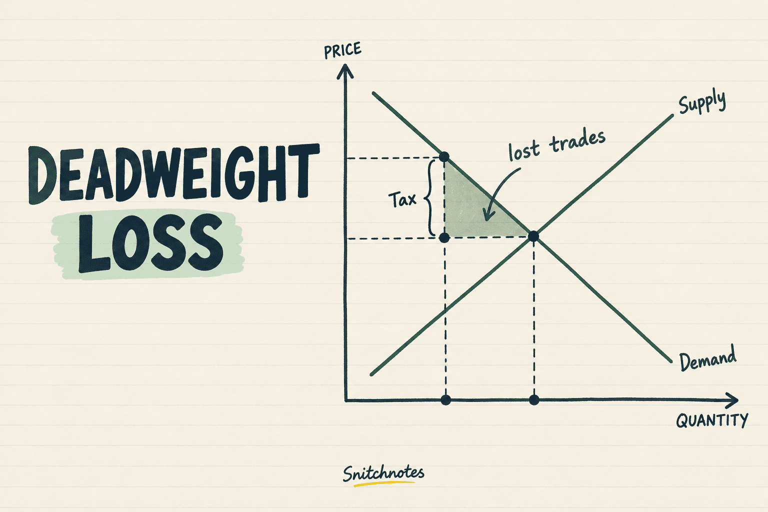
Deadweight loss is the reduction in total economic surplus that occurs when a market produces or trades an inefficient quantity. On a supply-and-demand graph, it is usually shown as a triangle between the demand and supply curves over the units that are no longer traded. Those units matter because buyers valued them more than they would have cost sellers to provide, yet the trades did not happen.

A tax is a classic cause: it creates a gap between the price buyers pay and the price sellers receive, reducing the quantity exchanged. This article builds one numerical example from equilibrium to the deadweight-loss calculation, then explains what the shaded triangle really means.

Why deadweight loss matters

Economists use total surplus as a compact measure of gains from trade. Consumer surplus is the difference between what buyers are willing to pay and what they actually pay. Producer surplus is the difference between the price sellers receive and their cost of supplying the good. At the competitive equilibrium in the standard model, all trades for which willingness to pay exceeds marginal cost take place, so total surplus is maximized.

MIT OpenCourseWare describes deadweight loss as a loss of welfare caused by moving away from the perfectly competitive equilibrium. The concept matters because it separates a transfer from a genuine efficiency loss. Money moved from buyers or sellers to the government is a transfer; the value of mutually beneficial trades that vanish is the deadweight loss.

Step 1: Find the no-tax equilibrium

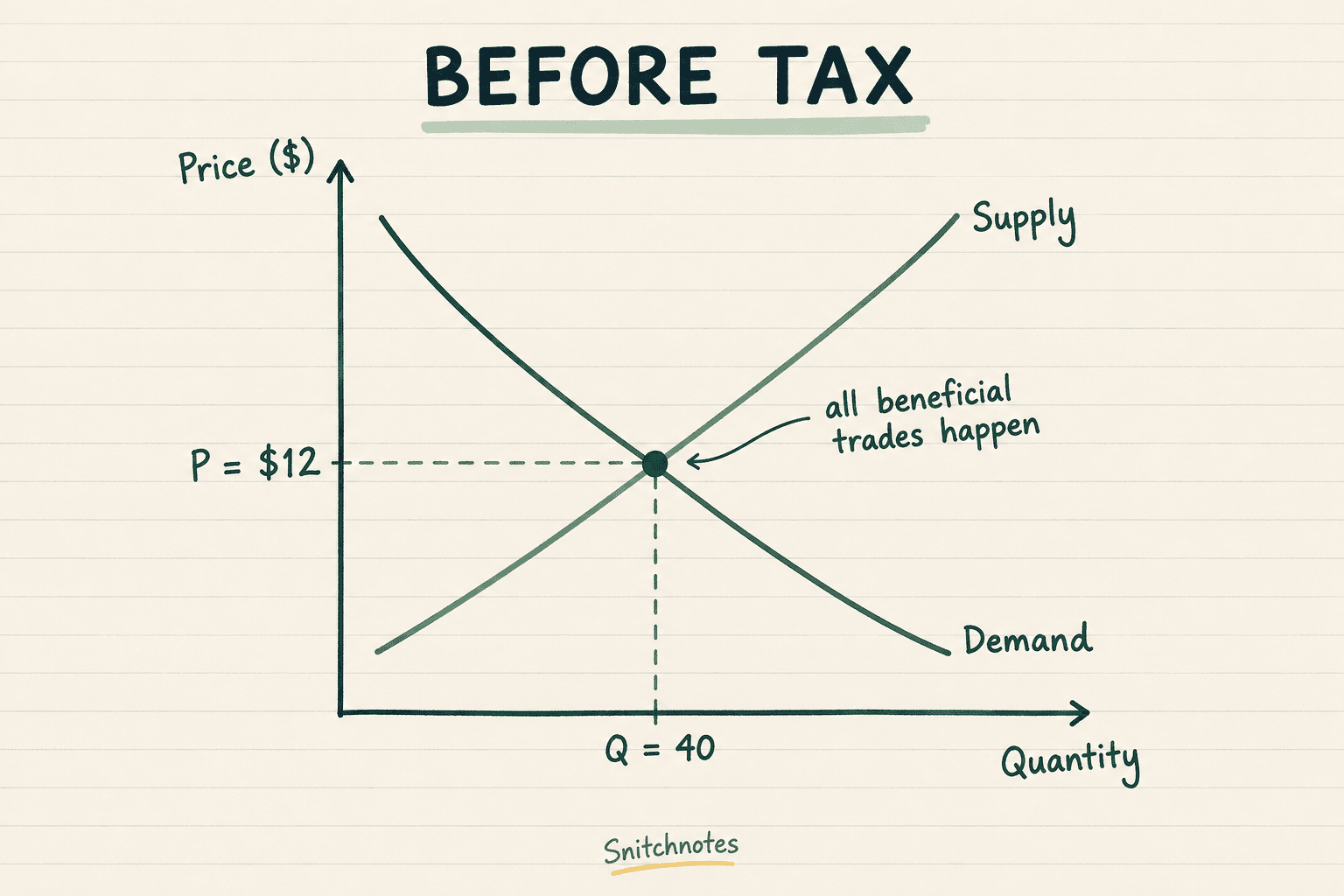
Suppose demand is P = 20 − 0.2Q and supply is P = 4 + 0.2Q, where P is dollars per unit and Q is units traded. Set demand equal to supply: 20 − 0.2Q = 4 + 0.2Q. Solving gives Q = 40, and substituting 40 into either equation gives P = $12.

This is the benchmark. Buyers purchase 40 units, sellers provide 40 units, and the market price is $12. The demand curve reaches $20 when quantity is zero, while the supply curve begins at $4. The total surplus is therefore the area of the large triangle between the curves: one-half × ($20 − $4) × 40 = $320.

Before tax, supply and demand meet at a price of $12 and a quantity of 40 units.

Step 2: Add the tax wedge

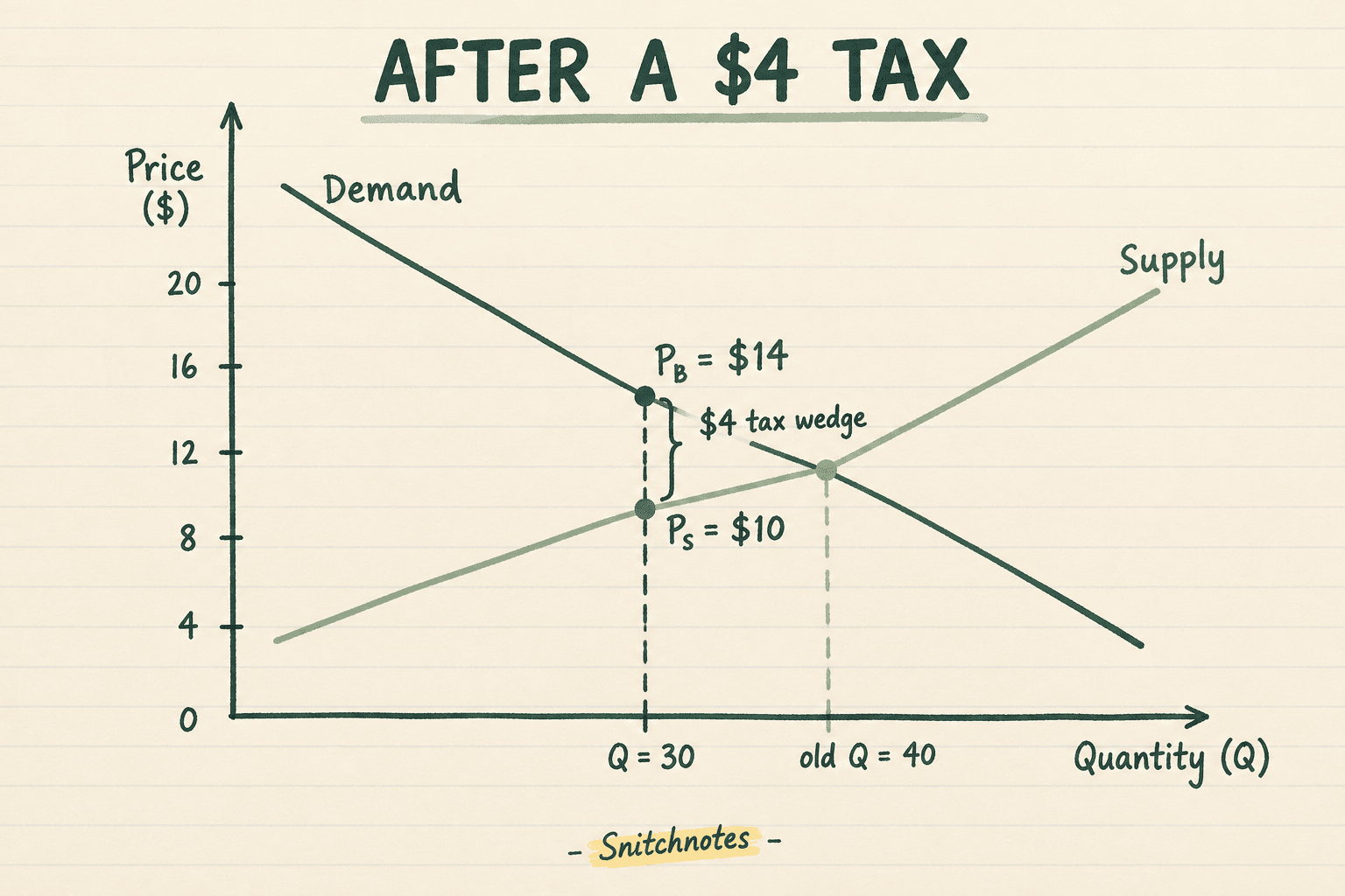
Now add a $4 tax on every unit sold. It does not matter for this graph whether the law says the buyer or seller sends the money to the government. What matters is the wedge: the buyer price must be $4 above the seller price. Write that condition as 20 − 0.2Q = 4 + 0.2Q + 4.

Solving gives Q = 30. Buyers pay $14 because 20 − 0.2(30) = 14. Sellers receive $10 because 4 + 0.2(30) = 10. The difference is the $4 tax, and tax revenue is $4 × 30 = $120. The important efficiency change is the fall from 40 to 30 units: ten previously beneficial trades disappear.

A $4 per-unit tax separates the buyer and seller prices and reduces quantity from 40 to 30 units.

Step 3: Calculate the deadweight-loss triangle

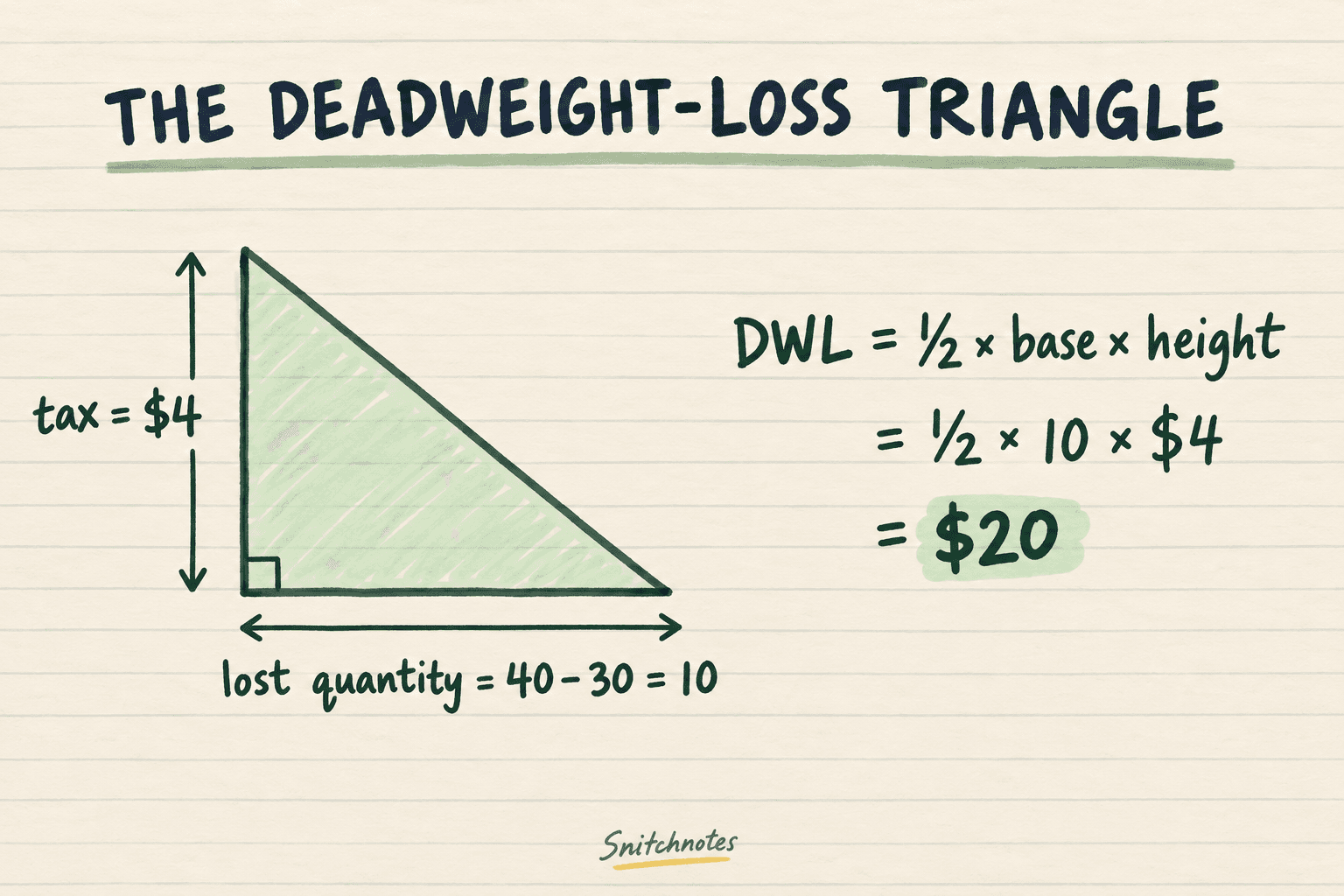
For straight supply and demand curves and a per-unit tax, the deadweight-loss area is a triangle. Its height is the $4 tax wedge. Its base is the reduction in quantity, 40 − 30 = 10 units. The calculation is DWL = one-half × tax per unit × reduction in quantity, so DWL = one-half × $4 × 10 = $20.

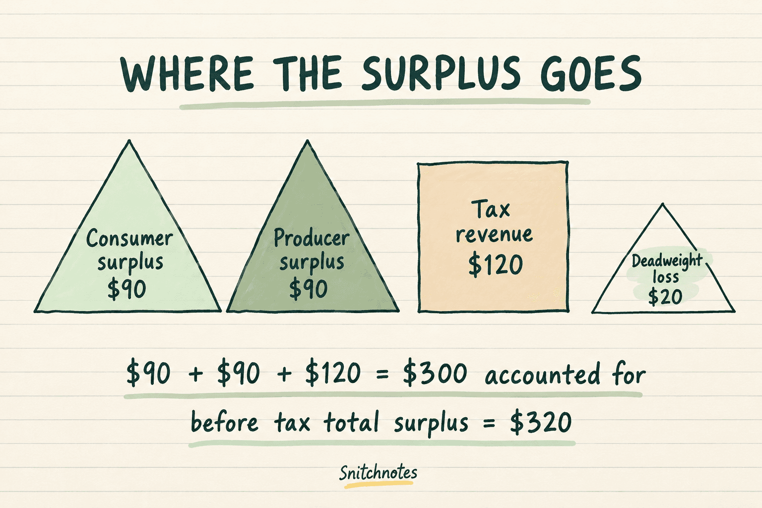
The same answer appears by comparing total surplus before and after the tax. Afterward, consumer surplus is one-half × ($20 − $14) × 30 = $90. Producer surplus is one-half × ($10 − $4) × 30 = $90. Add $120 of tax revenue and the total is $300. The original $320 minus $300 leaves $20.

The deadweight loss is one-half times the $4 tax wedge times the 10 lost units, or $20.

What the $20 loss does—and does not—mean

Deadweight loss is not the government's $120 of tax revenue. That money still exists and can finance services or be redistributed. Nor is it simply the combined drop in consumer and producer surplus, because part of that drop becomes revenue. The deadweight loss is only the surplus that nobody receives: the $20 associated with trades between quantities 30 and 40 that no longer occur.

The triangle also does not prove that every tax is bad. This basic graph counts the efficiency cost inside one market and assumes no external benefit or harm. A tax that corrects pollution can move output closer to the socially efficient quantity. Governments may also accept some efficiency cost to raise revenue or pursue fairness. Deadweight loss is one input to that decision, not the entire verdict.

After the tax, consumer surplus, producer surplus, and tax revenue total $300; the missing $20 is deadweight loss.

What determines the size of deadweight loss?

The more quantity responds to a tax, the more trades disappear and the larger the triangle becomes. That is why price elasticity matters. If buyers or sellers barely change quantity, the deadweight loss is smaller for a given tax wedge. If both sides respond strongly, quantity falls more and the loss grows. UC Berkeley's public-economics notes also show the standard result that, in the simple model, deadweight loss rises more than proportionally as the tax rate increases.

A useful exam rule is to find the efficient quantity first, find the actual quantity second, and then shade the area between demand and supply over the missing units. Do not automatically shade the tax-revenue rectangle. Rectangle equals transferred revenue; triangle equals lost surplus.

Consumer surplus: the gap between willingness to pay and the price paid.
Producer surplus: the gap between the price received and the seller's cost.
Price elasticity: how strongly quantity demanded or supplied responds to price.
Asymmetric information: how unequal knowledge can prevent efficient market outcomes.