
Snitchnotes Team
Price Elasticity vs Income Elasticity: Key Differences
Price Elasticity vs Income Elasticity: Key Differences
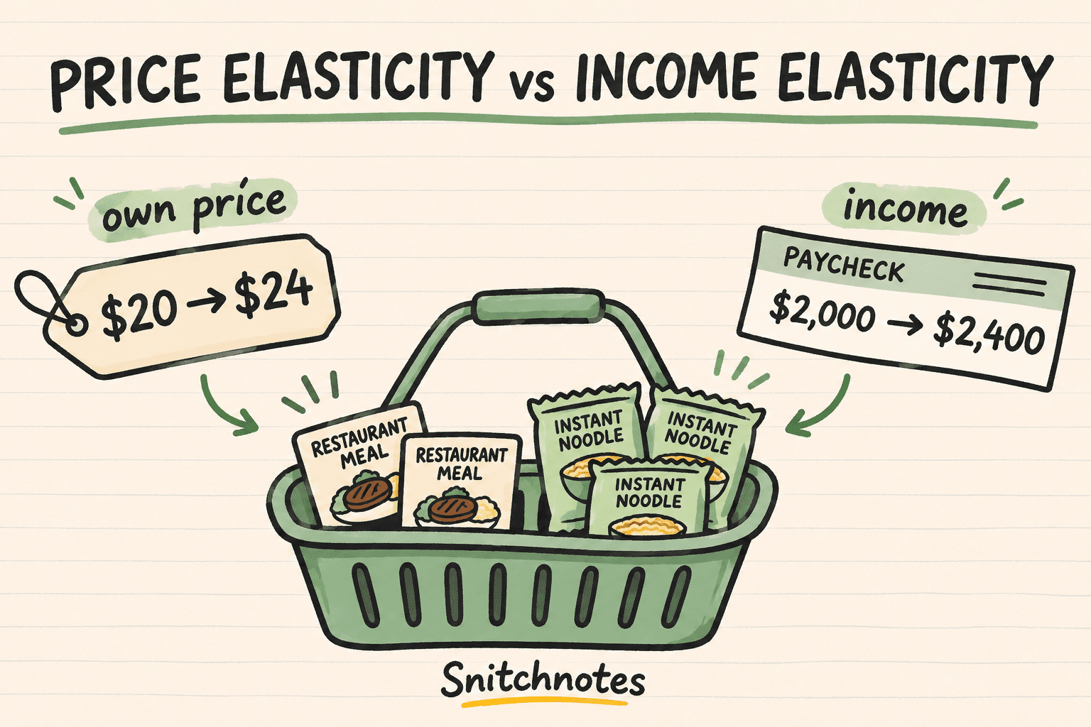
Price elasticity of demand measures how quantity demanded responds to a product's own price. Income elasticity of demand measures how quantity demanded responds to consumer income. Both use percentage changes and produce unit-free coefficients, but they answer different questions: price elasticity describes movement along a demand curve when the good's price changes, while income elasticity describes a demand shift when buyers' income changes.
The distinction matters whenever you interpret sales data or predict demand. A restaurant seeing fewer orders after raising its menu price faces a price response. A noodle brand seeing demand change as household incomes rise faces an income response. Mixing the two can lead you to use the wrong denominator, read the sign incorrectly, or call a good “elastic” in a way that hides what caused the response.
Price elasticity vs income elasticity at a glance
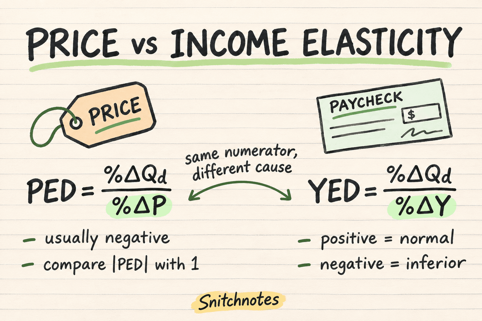
- Price elasticity of demand (PED): percentage change in quantity demanded divided by percentage change in the good's own price.
- Income elasticity of demand (YED): percentage change in quantity demanded divided by percentage change in consumer income.
- What changes: PED changes the product's price; YED changes purchasing power while the product's own price is held constant in the basic interpretation.
- What the sign tells you: PED is normally negative because price and quantity demanded move in opposite directions. YED can be positive or negative, classifying the good as normal or inferior over the measured range.
- What the magnitude tells you: the absolute PED value indicates whether demand is elastic, unit elastic, or inelastic. For positive YED, a value above 1 is commonly described as income elastic or a luxury, while a value between 0 and 1 is income inelastic or a necessity.
In short, PED asks, “How sensitive are buyers to this price?” YED asks, “How does demand change as buyers become richer or poorer?” The shared numerator can make the formulas look almost identical, so always name the variable in the denominator before calculating.
How to calculate both with the midpoint method
For any variable X changing from X₁ to X₂, the midpoint percentage change is (X₂ − X₁) divided by [(X₁ + X₂) ÷ 2], then multiplied by 100. Use that formula for quantity and for the relevant cause: price in PED or income in YED. The midpoint method uses the average of the two observations as its base, so reversing the direction of comparison does not change the elasticity's magnitude.
Then calculate PED = % change in Qd ÷ % change in P, or YED = % change in Qd ÷ % change in income. Keep the sign while doing the arithmetic. For PED, textbooks often report the absolute value when labeling demand elastic or inelastic; if you do that, say so. For YED, never drop the sign because it carries the normal-versus-inferior classification.
Worked midpoint examples
Restaurant meals: price elasticity
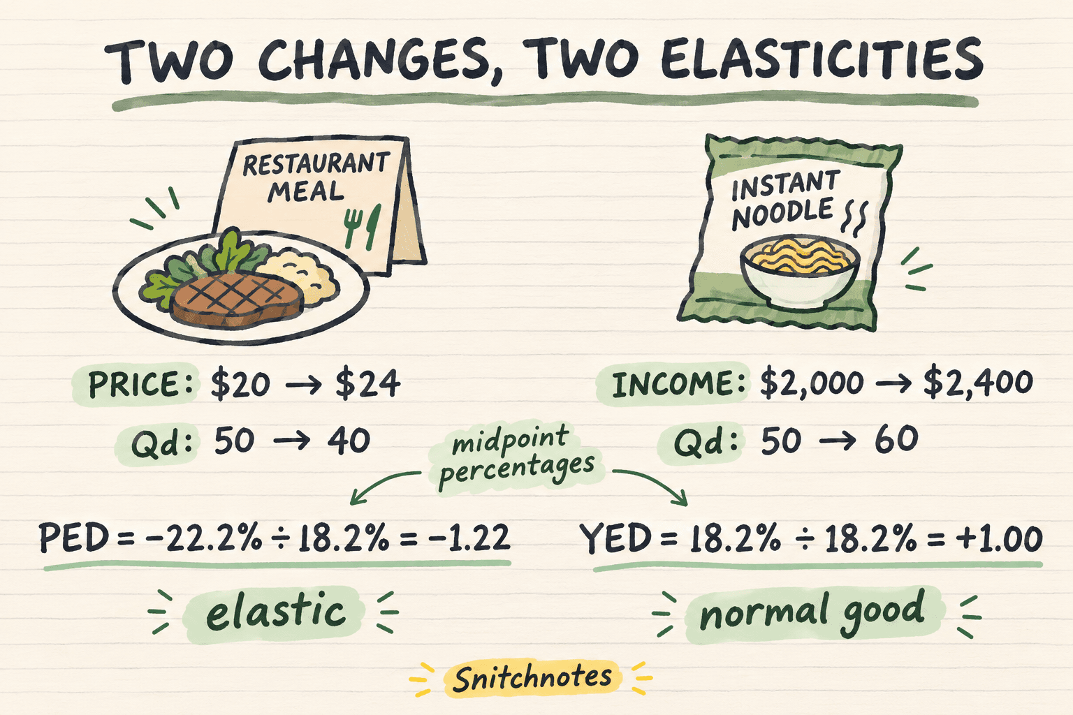
Suppose a restaurant raises a meal's price from $20 to $24 and quantity demanded falls from 50 to 40 meals per day. The midpoint quantity change is (40 − 50) ÷ 45 × 100 = −22.2%. The midpoint price change is ($24 − $20) ÷ $22 × 100 = 18.2%.
PED is −22.2% ÷ 18.2% = −1.22, or 1.22 in absolute value. Because the magnitude is greater than 1, demand is price elastic over this interval: quantity changed proportionally more than price. Daily revenue also falls from $1,000 to $960, which is consistent with a price increase when demand is elastic over the observed range.
Instant noodles: income elasticity
Now suppose monthly income rises from $2,000 to $2,400 while instant-noodle demand rises from 50 to 60 packs. The midpoint quantity change is (60 − 50) ÷ 55 × 100 = 18.2%. The midpoint income change is ($2,400 − $2,000) ÷ $2,200 × 100 = 18.2%.
YED is 18.2% ÷ 18.2% = +1.00. In this example, noodle demand is unit income elastic and the positive sign makes noodles a normal good for these buyers over this income range. Do not override the result with a stereotype: a product is not inherently inferior for every consumer, place, and income level. The classification comes from the measured relationship.
How to interpret signs and magnitudes
For ordinary downward-sloping demand, PED is negative. Use |PED| > 1 for elastic demand, |PED| = 1 for unit-elastic demand, and |PED| < 1 for inelastic demand. The sign usually confirms the law of demand; the magnitude carries the sensitivity label. Rare exceptions such as Giffen behavior require special conditions and are not the default assumption.
YED uses its sign and magnitude differently. YED > 0 identifies a normal good, while YED < 0 identifies an inferior good. Among normal goods, 0 < YED < 1 suggests demand grows less than proportionally with income, and YED > 1 suggests it grows more than proportionally. These are estimates for a particular market, population, and period—not permanent labels stamped onto products.
Common misconceptions and boundaries
First, elasticity is not slope. Slope compares changes in units; elasticity compares percentage changes, so it is unit-free and can vary along a straight-line demand curve. Second, a large positive YED does not mean demand is highly price sensitive. It means demand is highly responsive to income. Always attach the cause when you use the word “elastic.”
Third, the examples isolate one driver at a time. Real sales can change because of price, income, competitors, tastes, seasons, advertising, or expectations at once. A simple two-point calculation describes an association under the assumed ceteris paribus comparison; credible causal estimates need data and methods that separate overlapping influences.
Check your understanding
A product's price rises 10% and quantity demanded falls 5%. Which elasticity is this?
It is price elasticity of demand because the changing cause is the product's own price. PED is −0.5, or 0.5 in absolute value, so demand is price inelastic.
Income rises 8% and demand falls 12%. What does the sign mean?
YED is −1.5. The negative sign means the good is inferior for the measured consumers and range; the magnitude says demand changed more than proportionally to income.
Why use midpoint percentages?
They use the average of the starting and ending values as the base, avoiding different elasticity magnitudes depending on whether you describe the change forward or backward.
If elasticity formulas in your course notes keep blurring together, Snitchnotes can turn your lectures, PDFs, and notes into clearer study notes, quizzes, flashcards, and audio for practice.
Related concepts
- Price ceilings versus price floors: compare how legal price limits change market outcomes.
- Comparative advantage and opportunity cost: practice another core economics comparison with tables.
- Supply and demand shifting together: learn how to separate simultaneous market forces.
Sources
OpenStax, Principles of Economics 3e: Price Elasticity of Demand and Price Elasticity of Supply
OpenStax, Principles of Economics 3e: Elasticity in Areas Other Than Price
University of Minnesota Libraries, Principles of Economics: Elasticity—A Measure of Response
Georgia State University EconPort: Calculating Percentage Change
Federal Reserve Bank of St. Louis: The Price Elasticity of Demand and Celebrity Brands
Turn your lectures into exam-ready materials.
Notes, quizzes, podcasts, flashcards, and chat — from one upload.
Try your first note free